Trial Version Usage Walkthrough

QuickStart Demo Video (2min)

Full Usage Walkthrough Video (10min)

Step 1: Access Your Cluster

Use your username and password to sign into app.rapidfire.ai.

Go to the “Clusters” tab. You must see your trial cluster listed there along with URLs for the Jupyter notebook and Plutono dashboard, similar to the image below.

Step 2: Launch the Notebook

Upon opening the Jupyter Notebook link you should see the notebook home directory with the following 9 files: requirements.txt, rf_spec_imagenet.py, rf_spec_imdb.py, rf_spec_news.py, rf_spec_coco.py, rf-tutorial-imagenet.ipynb, rf-tutorial-imdb.ipynb. rf-tutorial-news.ipynb. rf-tutorial-coco-detseg.ipynb.

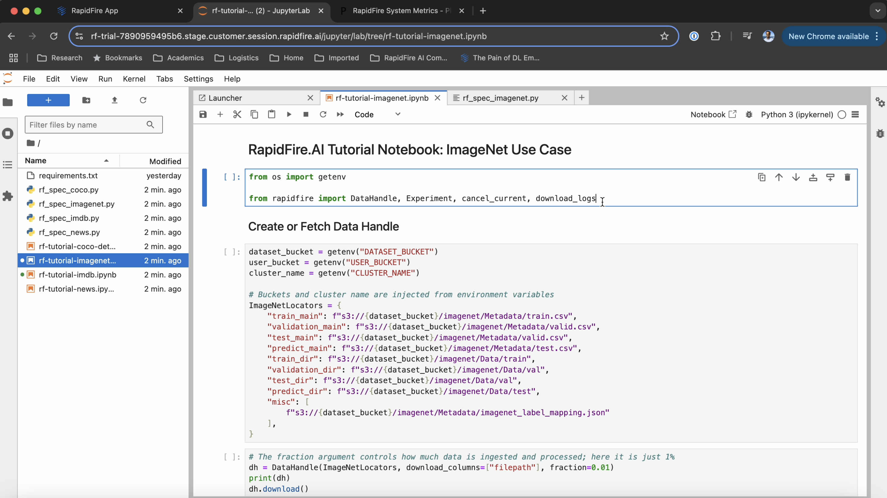
Open the tutorial use case notebooks and corresponding python code files illustrating the usage of our API. In particular, note how the MLSpec API is used to define the model, loss, and metrics.

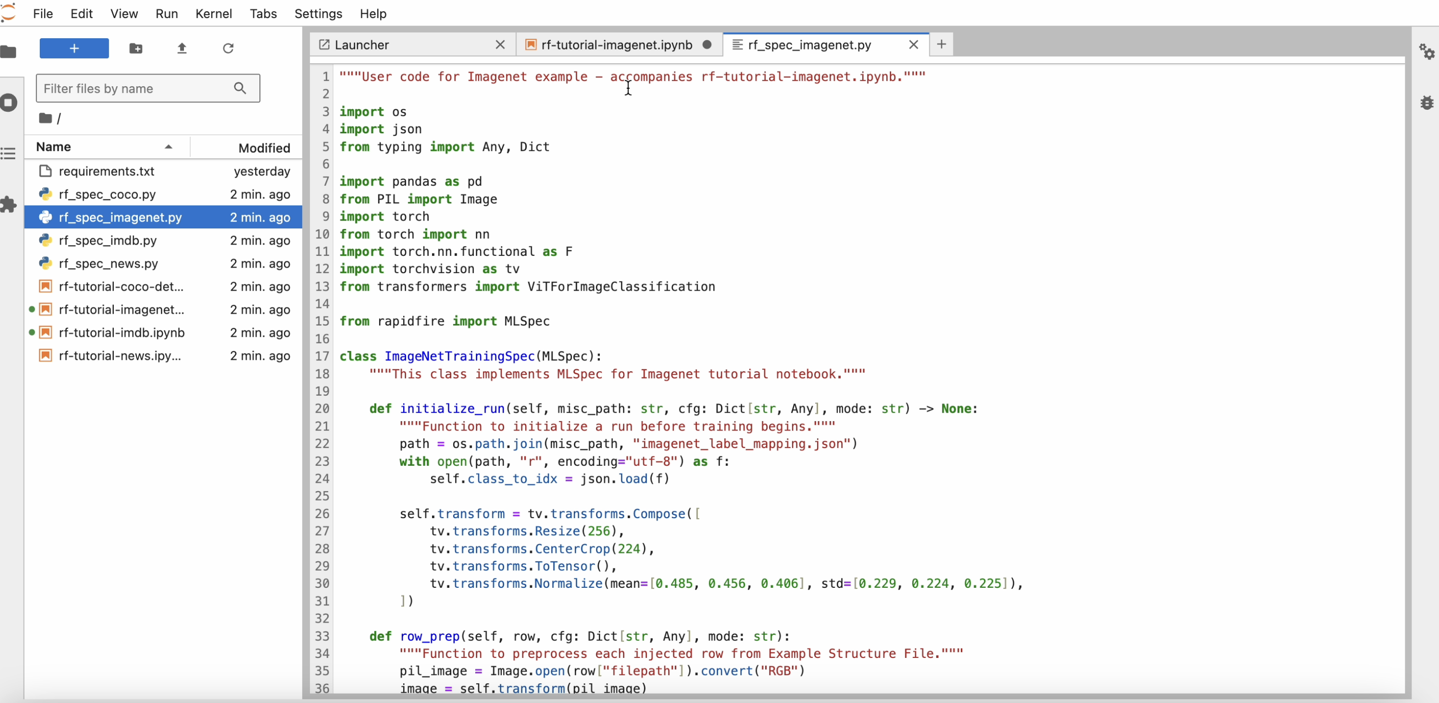
Check out the rest of this documentation website to explore our API and the product features further.

Step 3: Data Download

Start running the cells in one of the notebooks one by one. Please note that one cell must finish and return before you run the next cell.

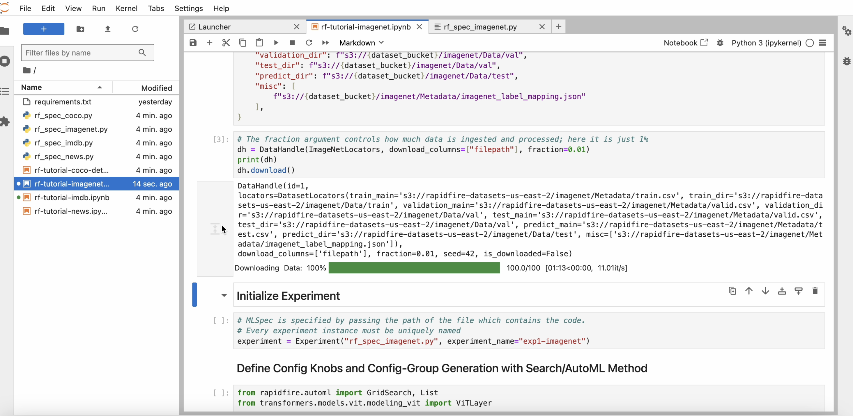
After you download() on the data handle, within a minute a progress bar will appear showing the percentage of data read from remote storage (S3 here) to your cluster.

Step 4: Create Experiment

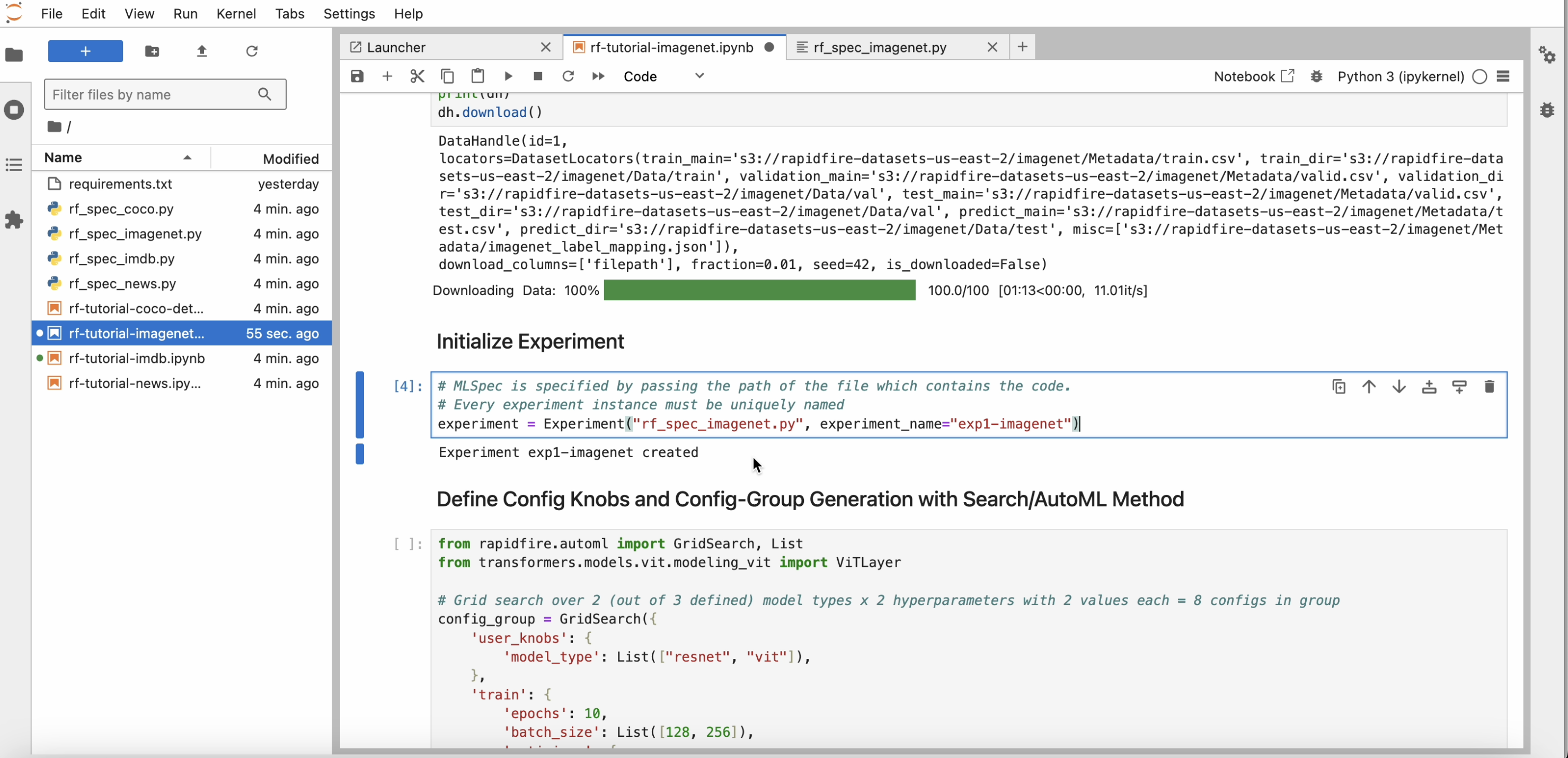
Run the cell with the experiment constructor and wait for the “experiment created” message to be printed. Note that every experiment created must have a unique name. If there is a name conflict, RapidFire AI will auto-extend the name.

Step 5: Launch Runs

Review the dictionary of configuration knobs; alter it if you’d like for the experiment, e.g., reduce the number of epochs or raise the number of hyper-parameters explored.

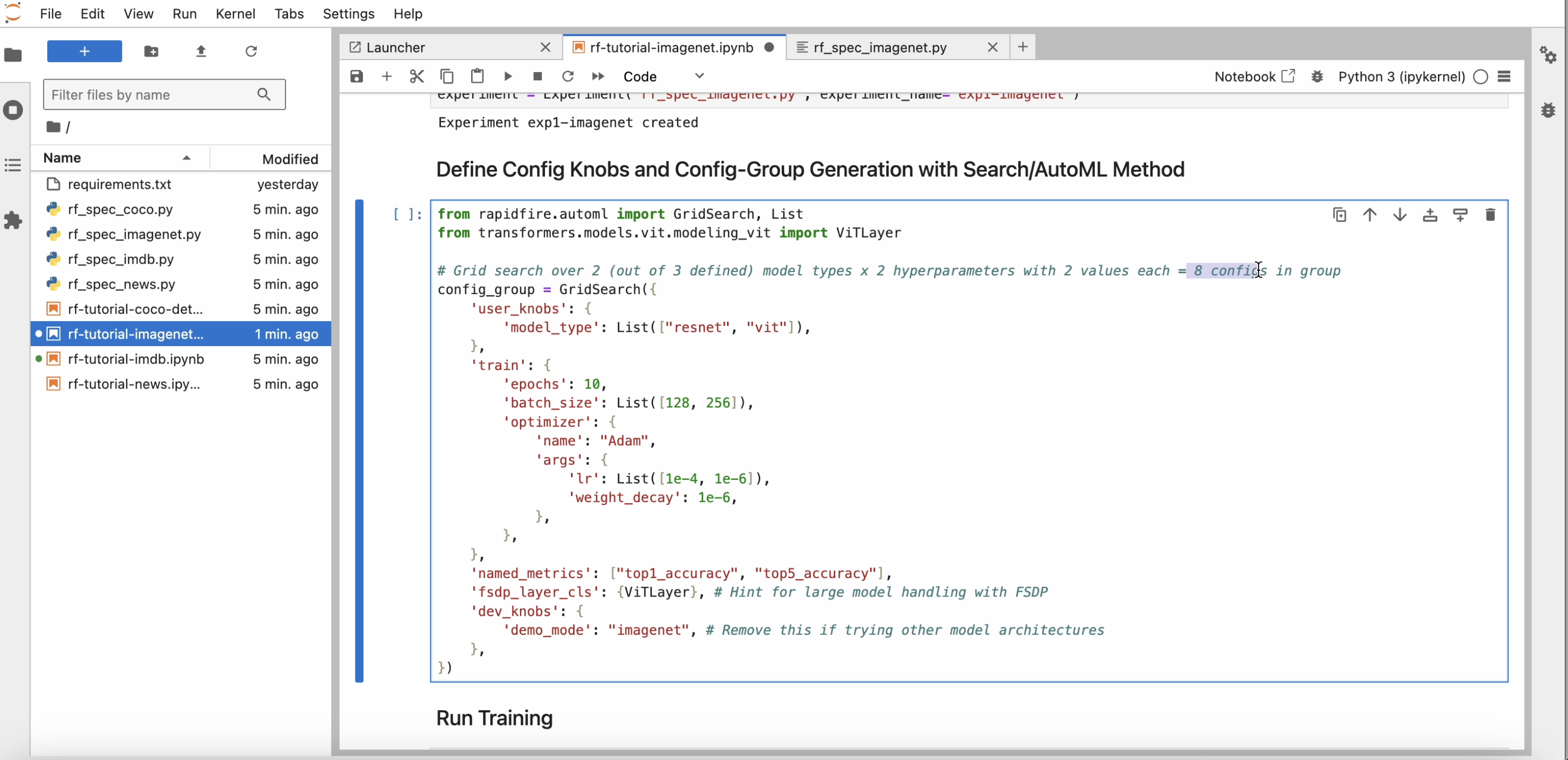
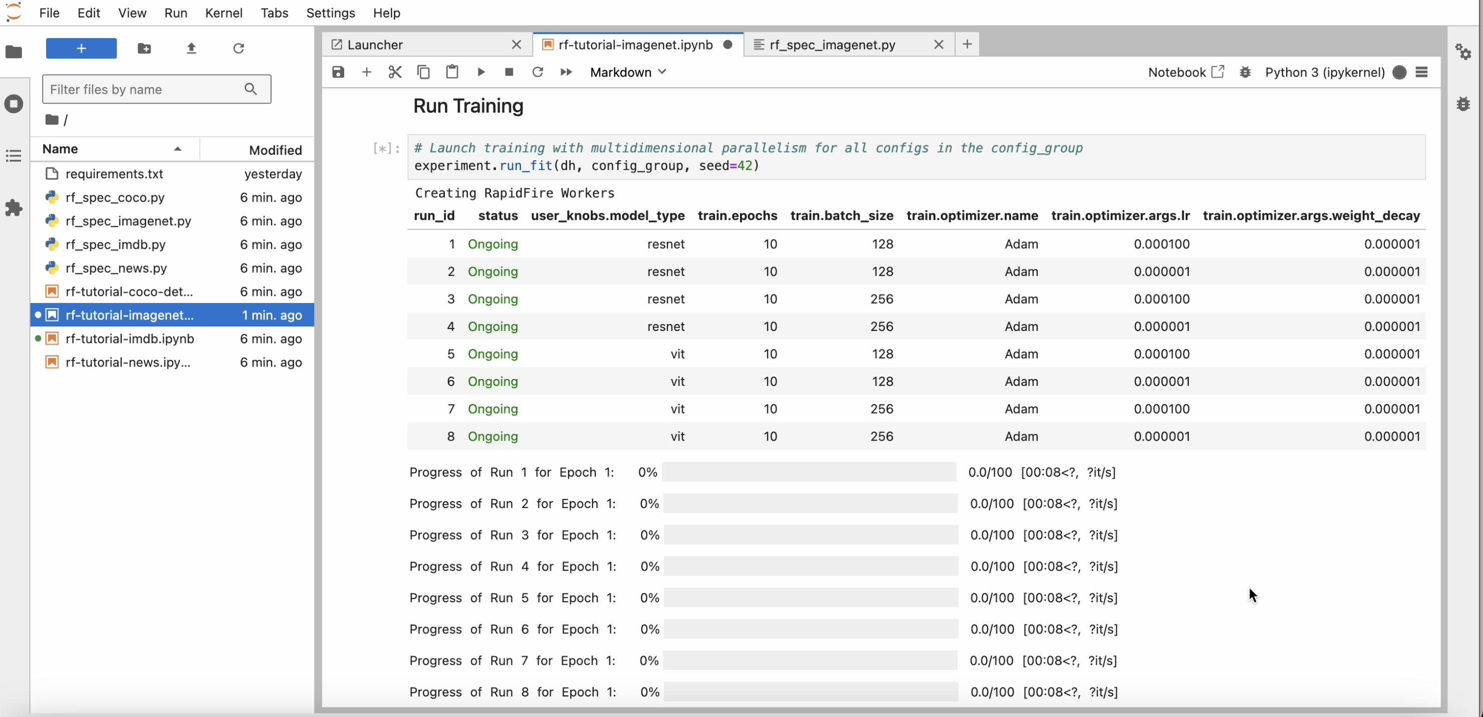
After you invoke run_fit(), within a minute or two the runs table and progress bars to appear. As the runs start learning, you should see progress bars for them as below.

Step 6: Monitor Training with ML Metrics Dashboard

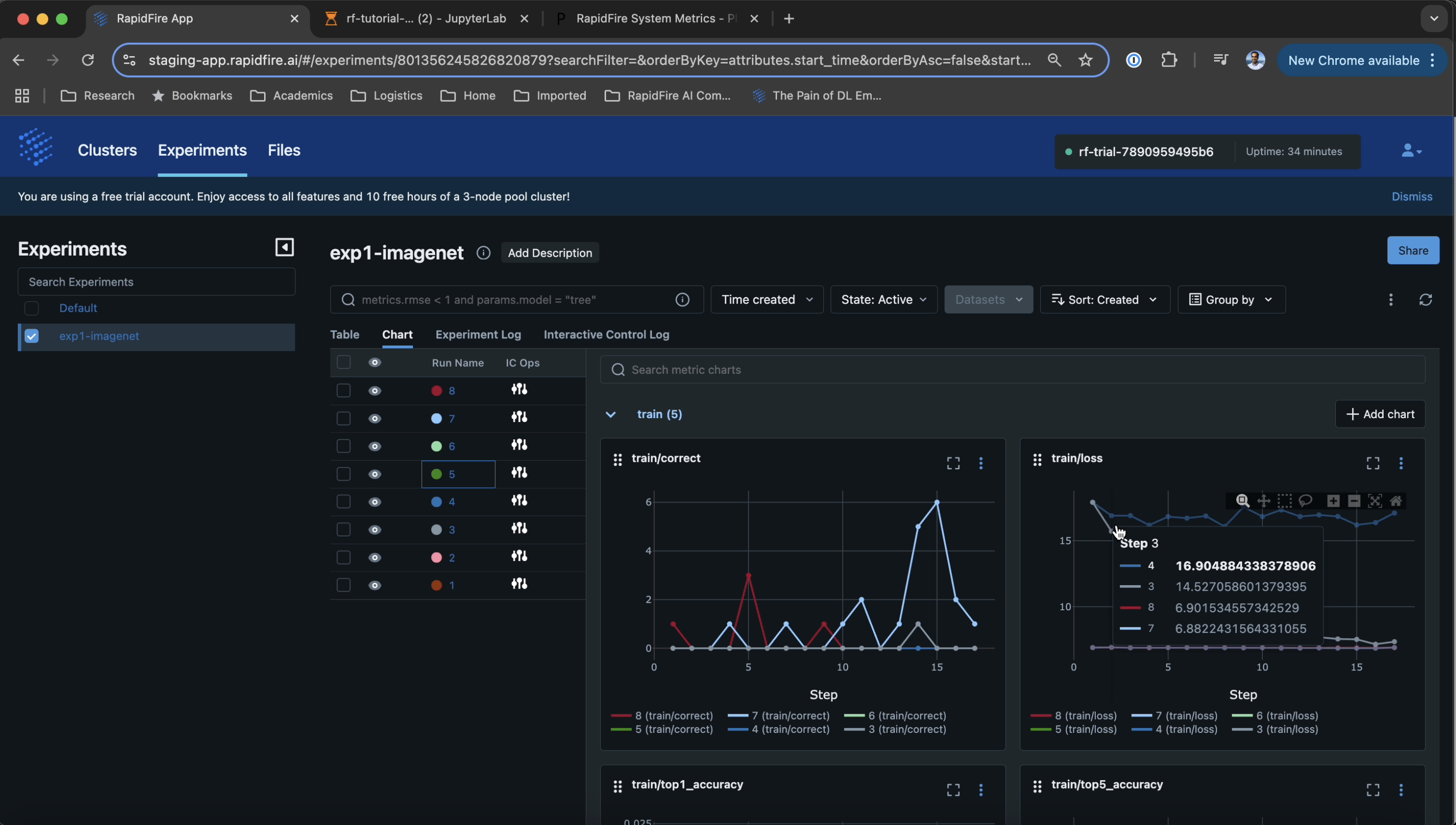
Once all runs have started learning a bit, head over to the RapidFire app again and click the “Experiments” tab and inside that page the “Chart” sub-tab. You should see all the metrics plots appearing automatically as below.

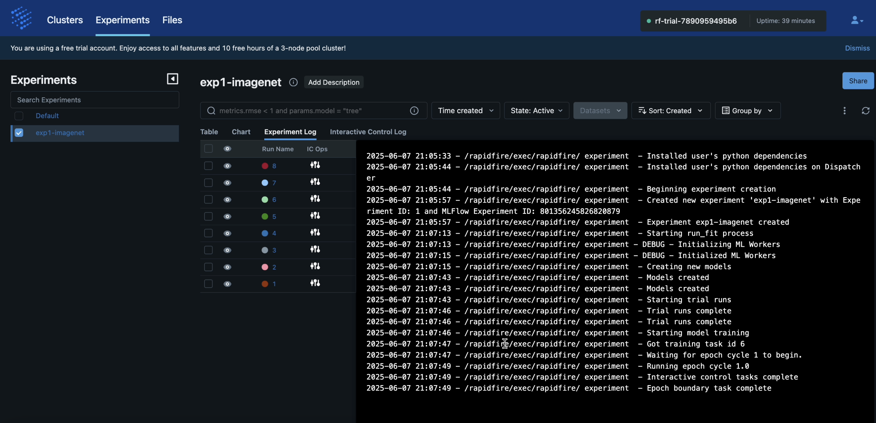
The experiment log keeps track of all the operations executed on your cluster.

Step 7: System Metrics Dashboard

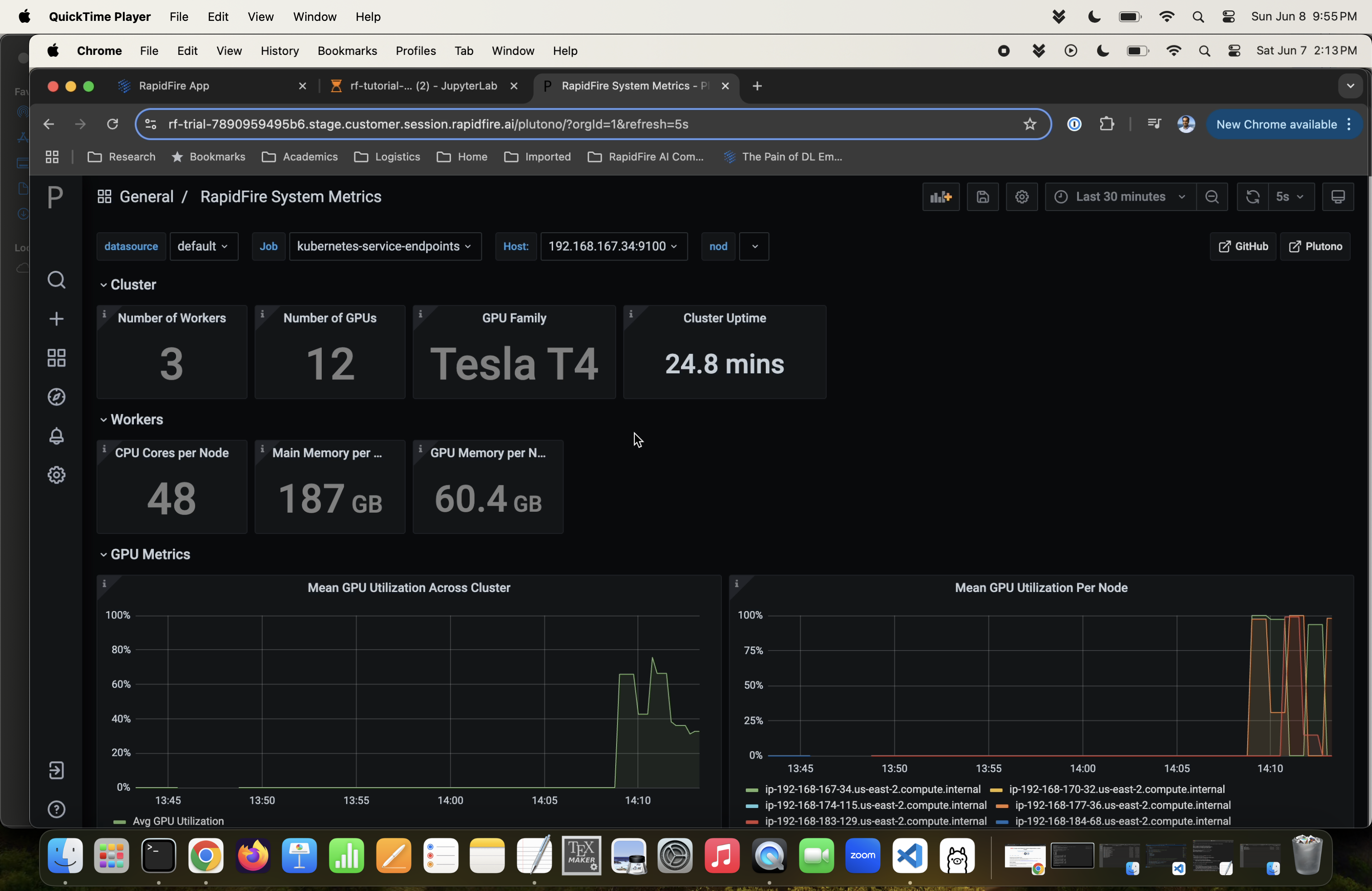
Click the “Clusters” tab and for your running cluster, click its “system metrics” dashboard URL. You will see a Plutono dashboard with all relevant GPU, CPU, DRAM, and other system metrics.

Step 8: Interactive Control (IC) Ops: Stop

Back on the RapidFire app page again, click the “Experiments” tab and inside that page the “Chart” sub-tab again. Click any one of the plots showing the runs, e.g., the “train/loss” plot, and expand its view using the relevant MLflow button.

The runs are likely to show disparate learning behaviors, some learning quickly (loss drops fast) and some learning slowly (loss stays high). Now we are going to perform some Interactive Control (IC) Ops on these runs as follows.

Step 8: Stop Run:

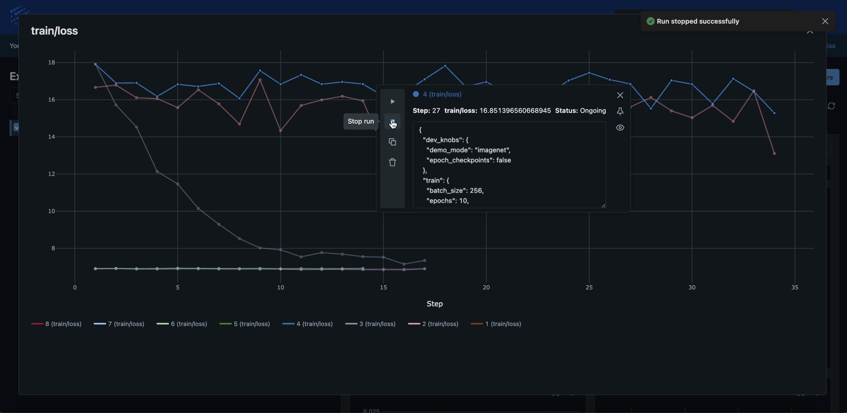
Click on a slow-learning run’s curve. The IC Ops panel should pop up. Now click the stop icon as shown below. You should see a “Run stopped successfully” message pop up on the top right of the page.

This IC op means this run has been slated for stopping at the end of this epoch. It will still remain alive and can be resumed later if you wish during the lifetime of this run_fit(). Likewise, the Delete button in the IC Ops panel removes that run altogether, i.e., it cannot be resumed later.

Step 9: IC Ops: Clone-Modify

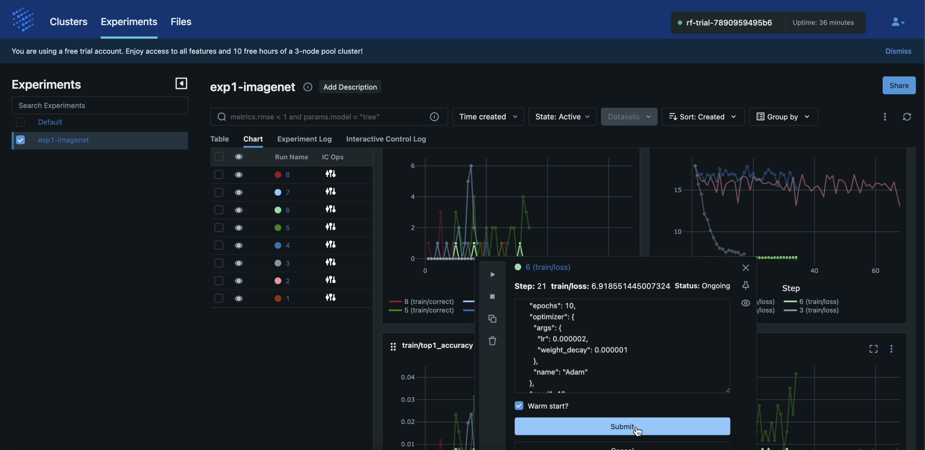
Now click on a fast-learning run’s curve. The IC ops panel should pop up again. Click the copy icon as shown below. A text box showing the run’s full config will become editable.

Inside that text box, alter any config knobs as you wish, e.g., the learning rate hyperparameter (a train knob) or image resizing (a user knob) based on your accuracy intuition about the use case, dataset, and model at hand. You can also include a new config-group generator, e.g., GridSearch(), or just provide a single new config. These result in “clone” runs of the chosen run with your newly specified knob values.

In the example shown below, we are adjusting the learning rate to add a single new clone. Note that you can “warm start” the clone’s model weights if you like–note that this will throw an error if your model architecture is not preserved for the clone.

Click the “Submit” button. You should see a message saying “Run cloned and modified successfully” pop up on the top right.

Step 10: Check Results of IC Ops

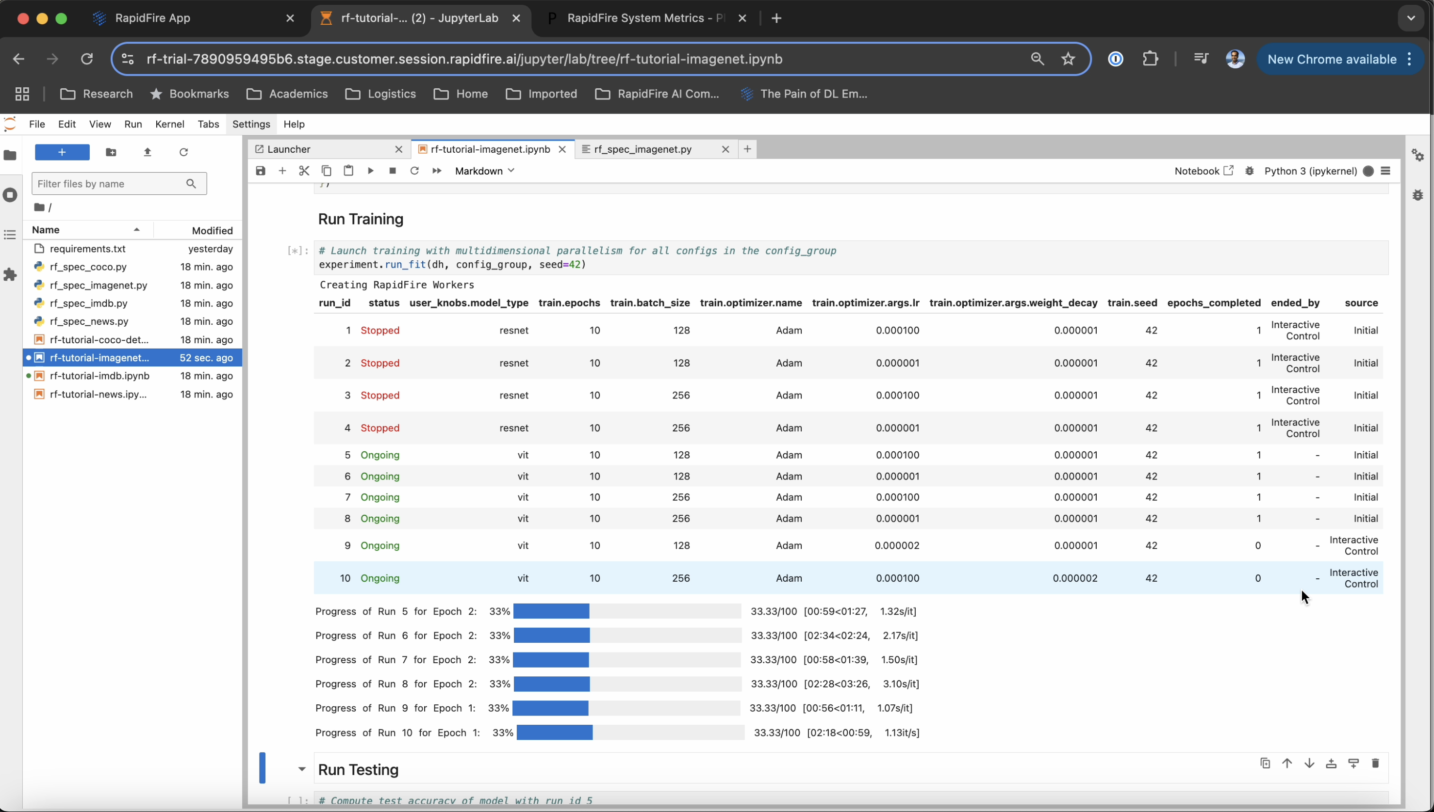
Once the ongoing epoch ends for all runs, all your IC Ops will be applied back to back. Head back over to the Jupyter Notebook for the run status table and progress bars. You should see the runs you had stopped/deleted have their status change to that. Likewise, the clones will also have new entries in the table.

Back on the ML metrics dashboard, the clones will have their curves appear automatically on the metrics plots as shown below.

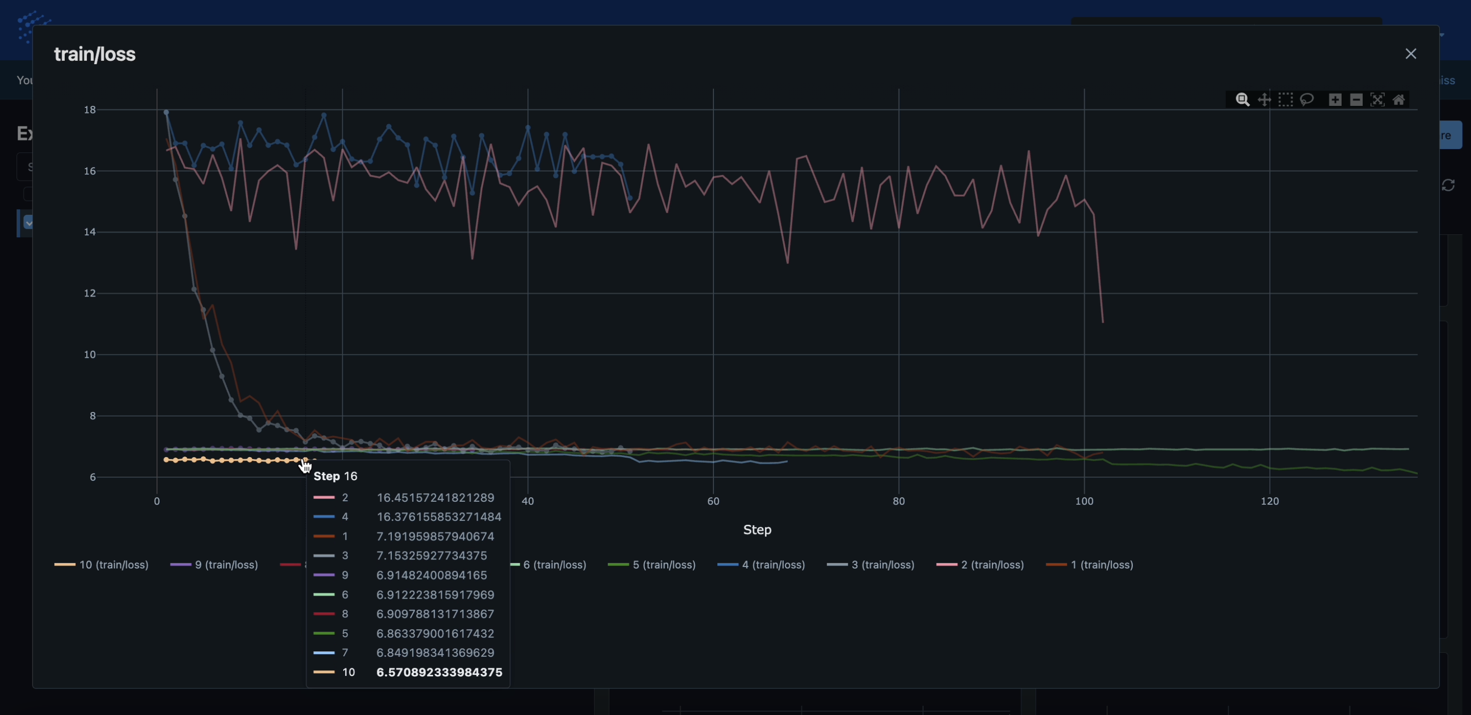
Under the hood, RapidFire AI’s multidimensional-parallel engine automatically re-allocates GPUs across workers to the active runs after all the IC Ops in a resource-optimal manner. So, you do NOT need to worry about the hassle of manually reallocating GPUs, waiting for jobs to finish, launching separating jobs or clusters, etc.

Play around with more IC Ops for as long as you wish, e.g., Resume the the runs you stopped earlier, clone the clones further, and so on. Your imagination is the limit! Such agility for rapid experimentation sets RapidFire AI apart from all other tools, and it will help you reach a much better accuracy much sooner.

Step 11: Test, Predict, and End Experiment

After run_fit() finishes fully (including your IC Ops), head back over to the Notebook. Now invoke run_test() to see the test set accuracy for a chosen run. Likewise invoke run_predict() and see the prediction outputs in the file that is returned and linked.

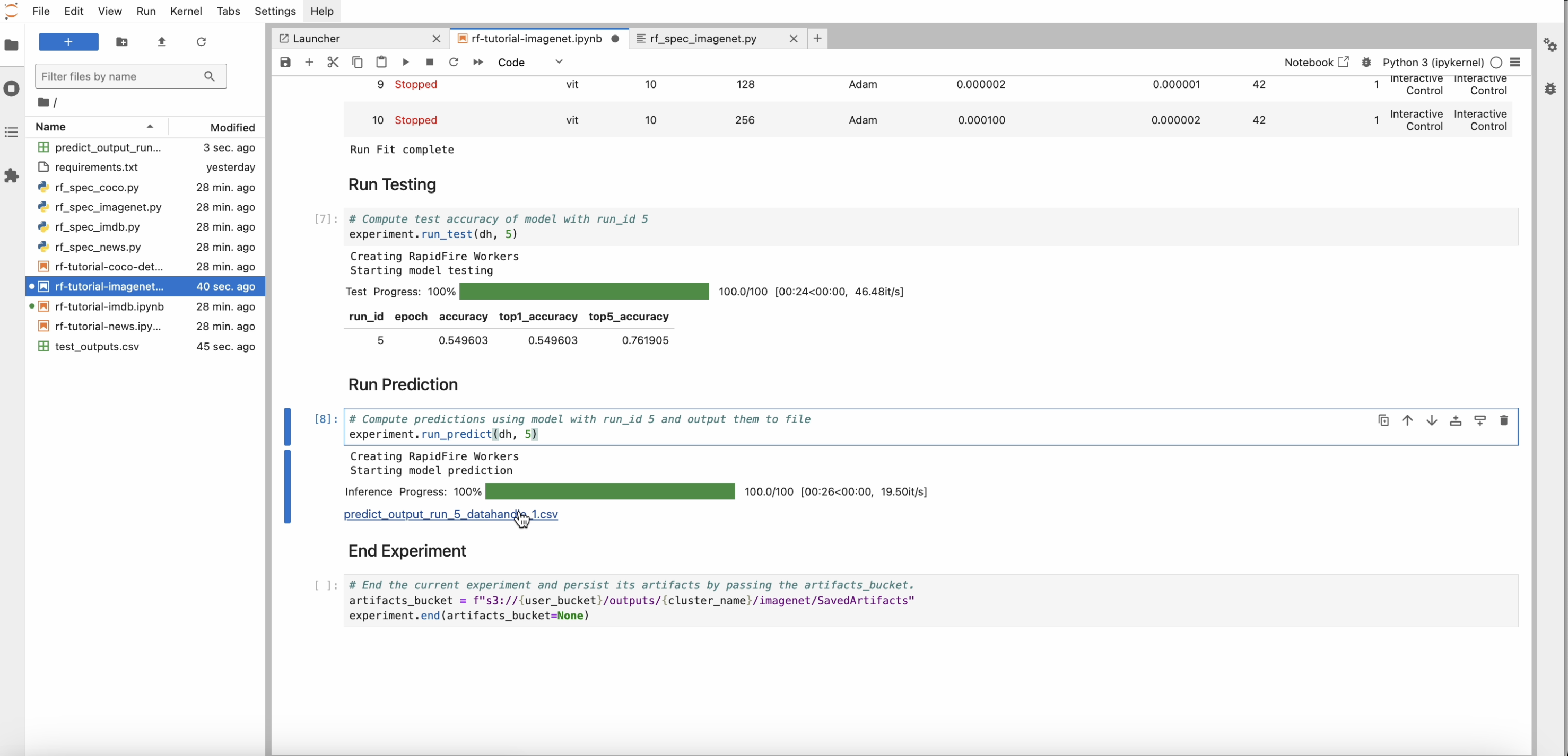
Finally, end_experiment() ends this experiment session. Optionally save all artifacts produced–model checkpoints, metrics files, information logs, and test or prediction outputs–to an S3 bucket.

Step 12: Venture Beyond!

After trying out all the tutorial use case notebooks, check out the rest of this documentation webpage, especially the API and dashboard docs. Perform more operations and experiments as you wish, including changing the MLSpec code and config knobs.

To upload your own dataset or model files, head over to the “Files” tab on the app. The zipped folder you provide there will be unzipped and saved on your allocated S3 bucket. Indicate whatever structure you want for that folder. Then list those S3 paths suitably in your new Data Handle locators for your new experiments.